2. Theory
2.1. Introduction
Magnetic clouds (MCs) are highly magnetized plasma structures that have a low proton temperature and a magnetic field vector that rotates when seen by a heliospheric observer. As motivation MC are the most geo-effective structures in the Interplanetary medium. Even though MCs have been studied for more than 25 years, there is no agreement about its true magnetic configuration. This is mainly because the magnetic field data retrieved in situ by a spacecraft correspond only to the one dimensional cut along its trajectory and, thus, it is necessary to make some assumptions to infer the cloud 3D structure from observations. Magnetic Clouds have been locally considered as cylindrical symmetric structures. From in situ observations and assumptions on the magnetic distribution inside the MC, it is possible to estimate some global magnetohydrodynamic quantities, such as magnetic fluxes and helicity for instance. In order to obtain good estimations of these quantities,it is necessary to find the correct MC orientation, and improve the estimation of its size and components of B in the cloud frame.
The Minimum Variance method (MV) has been extensivelyused to find the orientation of structures in the interplanetary medium. The Minimum Variance method applied to the observed temporal series of the magnetic field can estimate quite well the orientation of the cloud axis, when the distance between the axis and the spacecraft trajectory in the MC (the impact parameter, p) is low with respect to the cloud radius. The MV method has two main advantages with respect to other more sophisticated techniques that are also used to find the orientation of an MC: (1) it is relatively easy to apply, and (2) it makes a minimum number of assumptions on the magnetic configuration, only local cylindrical symmetry (so it is model independent). When p is significant,the MV approach provides orientations with more error from the real ones, and these errors can be estimated as well .In Section 1, we describe briefly the Minimum Variance method applied to magnetic clouds under the hypothesis of locally cylindrical symmetric configurations.
2.2. Section 1
In this section the Minimum Variance Technique is explained,how it is applied to magnetic clouds type structures in the interplanetary medium and the advantages of the technique.
2.3. Minimun Variance Technique
2.3.1. The Method
The MV method finds the direction n in which the projection of a series of N vectors has a minimum mean quadratic deviation and also provides the directions of intermediate and maximum variance. This method is very useful to determine the orientation of structures that present three clearly distinguished variance directions. In particular, when this method is applied to the magnetic field B, the mean quadratic deviation in a generic direction n is:
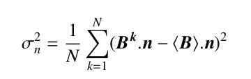
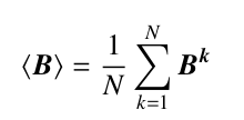
here B^k corresponds to each element k of the magnetic field series. The field mean value is
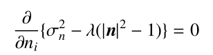
The MV method finds the direction where sigma_n^2 is minimum under the constraint mod(n)=1 . The Lagrange multipliers variational method can be used in this determination lambda is the Lagrange multiplier in the following system of equations:
where i=1,2,3 corresponds to the 3 components of n. After applying Eq.(3), the resulting set of three equations can be written in matrix form as:
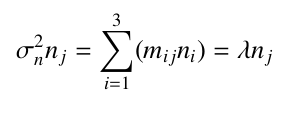
where
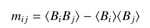
The indexes i,j represent the field components. The matrix mij is symmetric with real eigenvalues lambda1, lambda2 and lambda3 and orthogonal eigenvectors (Xmv, Ymv, Zmv), which represent the directions of minimum, maximum and intermediate variation of the magnetic field (the symbol’’^’’) on top of a variable means that it is a unit vector). The eigenvalues provide the corresponding variance sigman^2 associated with each direction. Thus, from the eigenvectors (Xmv, Ymv, Zmv),it is possible to construct the rotation matrix T such that the components of the field in the MV frame of reference can be written as:
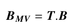
We will call BxMv the field component that corresponds to Xmv (minimum variance direction), BYmv to that of the maximum variance direction, and BZmv to that having the intermediate variance.
2.3.2. Minimun Variance method applied to magnetic clouds
The large and coherent rotation of the magnetic field vector observed by the spacecraft when p ~ 0, allows us to associate: (1) the large scale maximum variance direction to the azimuthal direction (variation of the observed component of the field of the order of 2 B0, for Bphi component, (2) the minimum variation to the radial direction (the variance will be close to zero, for the radial Br component, and (3) the intermediate variance to the axial direction (variation of the order of B0, or the axial Bz component, the observations of magnetic clouds, show that the modulus of the magnetic field does not remain constant, being maximum near the cloud axis and minimum toward the cloud boundaries. Moreover, for MCs in expansion and due to magnetic flux conservation in the expanding parcels of fluid, mod(B) can decrease significantly while the spacecraft observes the cloud. This decrease of mod(B) with time is called the ‘aging’ effect since the {it in situ} observations are done at a time, which is more distant from the launch time as the spacecraft crosses the MC. This decrease of mod(B) can affect significantly the result of the MV method. However, the relevant information to find the cloud orientation is in the rotation of the magnetic field. Thus, to decouple the variation of mod(B) from the rotation, we apply the MV technique to the normalized field vector series: b(t) = B(t)/mod(B(t)). Because MV does not give the positive sense of the variance directions, we choose his sense for Xmv so that it makes an acute angle with the Earth-Sun direction (Xgse). We also choose Zmv so that Bzmv is positive at the cloud axis, and Ymv is closing the right handed system of coordinates. The intrinsic cloud reference system and the Geocentric Solar Ecliptic (GSE) system of coordinates can be related using the following rotation matrix:
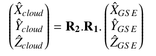
where:
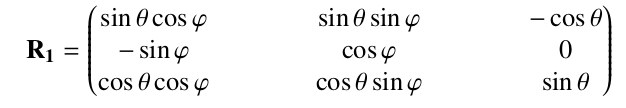
and
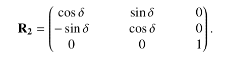
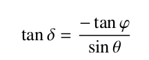
Without loosing generality we choose delta (the angle of an arbitrary rotation in the plane (Xcloud, Ycloud) such that Xgse.Ycloud = 0, that is:
In this way we can apply the technique to the parcel of Solar Wind that corresponds to an MC and rotate it in the Cloud Frame.
2.4. Section 2
In this section we describe the development of the project identified with our logo Figure 1. The aim was to produce a package publicly available to find the orientation of a MC and rotate it to its local frame. We changed the functions pipe-line structure of our matlab previous implementation to the Object Oriented Programming Python paradigm (since Python is a programming language Turing-complete) to provide a package easy to install and run, with an open source repository, providing quality standards to reach a wider community of astrophysicists and astronomers interested in heliophysics and Sun-Earth relationship. Taking into account that a Magnetic Cloud has its own identity, state or attributes and behavior (relationships and methods), the Python paradigm was in order. As can be seen at Figure1 we designed an easy to identify logo for the project as well. Since there were no APIs to find the MC axis orientation implemented in Python and freely offered, we regard our project as a valuable contribution to the heliophysics community.
2.5. Aknowledgements
A.M.G. is member of the Carrera del Invesigador Cientifico, CONICET.